The False Positive Trap: The Dark Side of Bayesian A/B Testing

In my last post on surviving the “haircut”, I explored how Bayesian A/B testing handles corporate conservatism. The simulation showed that you can apply a massive 50% discount to your historical data and still beat a standard Frequentist test in low-traffic environments.

But there is a natural follow-up question. If we use a history of winning features to boost our power, what happens when we test a bad idea? Doesn’t an optimistic prior drastically increase our false positive rate for future duds?

I ran a new simulation to find out.

A quick note on terminology: strict Bayesians may not typically use Frequentist terms like power or false positive rate. But business stakeholders care about the long-run frequency of correct ship and no-ship decisions, so I am using these applied equivalents to benchmark the two methods.

The setup: the dud and the harmful feature

I kept the exact same low-traffic parameters, N=300 per arm, but decoupled the history from the new experiment:

• The optimistic history: k past experiments that were genuine winners, at a true +2.0% lift.
• The dud feature: a new experiment where the feature does absolutely nothing, a true 0% lift.
• The harmful feature: a new experiment that actively degrades the user experience, a true −1.0% lift.

I then applied the same stakeholder haircuts, from 0% to 100%, to the prior mean to see how often the Bayesian model would incorrectly push these bad ideas as a ship.

The cost of an optimistic prior

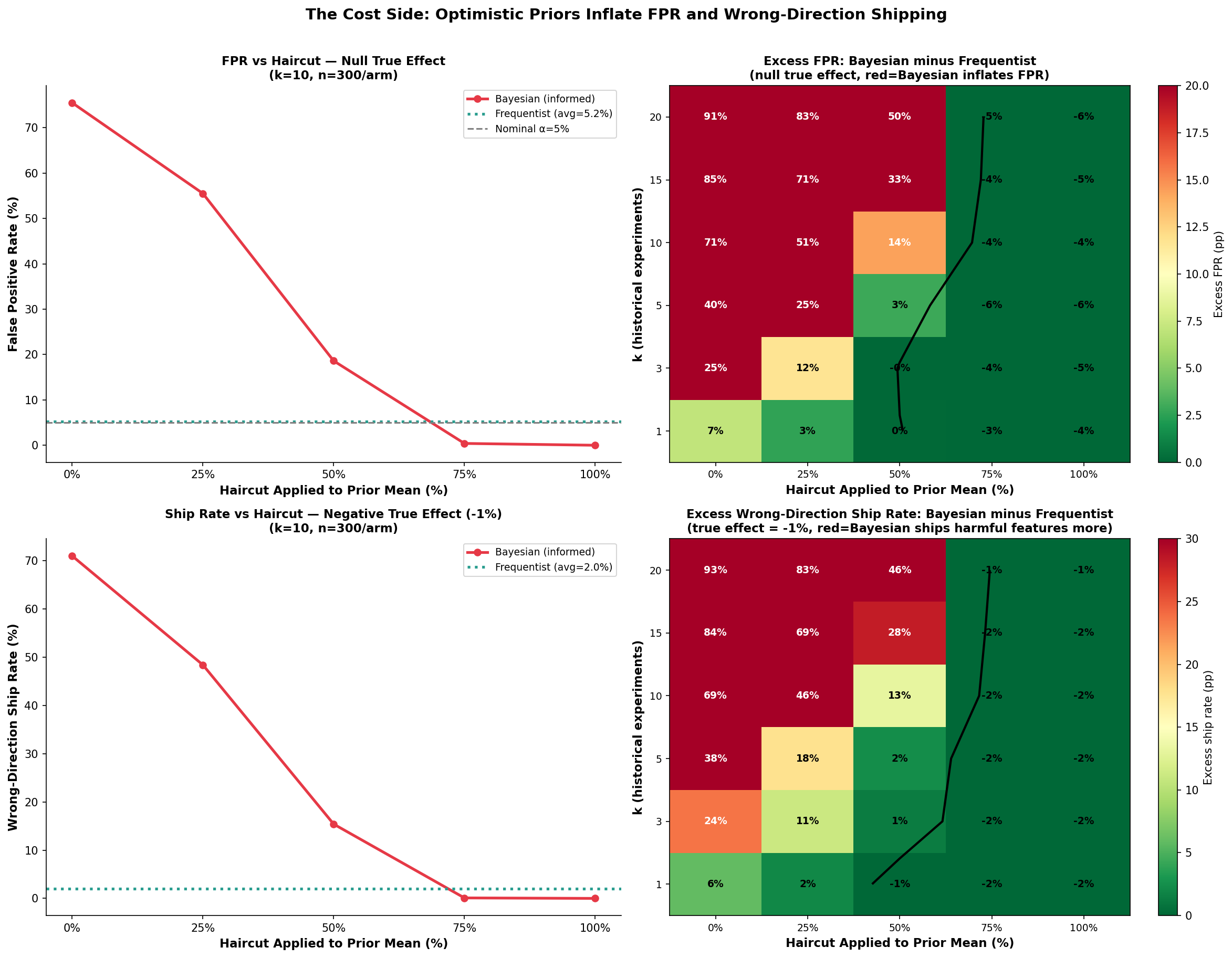
1. Bayesian power isn’t magic, it’s a wager. Frequentist tests have a fixed, nominal false positive rate of about 5%. Bayesian models do not. By using an optimistic prior, you are mathematically choosing to accept a higher false positive rate on bad ideas in exchange for higher power on good ones.

2. Blindly trusting history is a massive trap. If you have k=10 historical winners and apply no haircut, your false positive rate skyrockets to 75%. The model is so anchored to past success that it blindly approves the new dud.

3. Optimistic priors can ship harmful features. Testing a feature that actively loses money at −1% lift, with a small sample, the new negative data struggles to overcome the positive history. At k=10 with no haircut, you have a 71% chance of accidentally shipping a harmful feature.

4. The 50% haircut is a vital safety net. In the previous post, a 50% haircut preserved statistical power. Here it also acts as a shield: at k=10, conceding it drops the false positive rate from 75% to a much safer 18.6%, and the harmful ship rate to just 15.4%.

The bottom line

If you are operating in a low-traffic environment and using Bayesian priors, you have to be careful about regime changes. If your product suddenly stops producing easy wins, an optimistic prior will cause you to ship a wave of duds.

Applying a conservative haircut to your history isn’t just about appeasing a skeptical finance team; it is an important statistical safety net. There’s a critical tradeoff between higher ship rates for small positive effects and safeguards against shipping harmful changes.

If you’ve tackled this kind of regime change in production, I’d love to hear what safeguards your team uses when historical win rates start to dry up.