Don’t Trust the Closed-Form: Sizing Switchback Experiments with Permutation Tests

If you operate in a rigid marketplace environment like Amazon, standard user-level A/B testing is infeasible. You cannot randomize bids at the individual user level; every customer searching a specific keyword sees the exact same auction results.

In a previous experiment I bypassed this walled garden by building an automated daily switchback pipeline. Because we couldn’t randomize users, we randomized time. By toggling my Amazon ad bids up and down on a daily schedule, I found the true incremental value of the ads and ultimately slashed my ad spend by 69% while improving net profit.

Moving from user-level A/B testing to time-series experimentation introduces a dangerous statistical trap. To size an experiment like this properly, we have to talk about why standard closed-form asymptotic math fails on short switchbacks.

The big-data illusion and the i.i.d. trap

In a daily switchback experiment, your unit of randomization is the day itself.

The trap is that you may observe hundreds or thousands of sales and clicks every single day, which makes it feel like high-powered big data. But because the treatment is applied to the entire day, the variance of individual shoppers collapses into a single daily aggregate. If you run a two-week test, your effective sample size is exactly N=14.

SE = σ × √(1/n_t + 1/n_c)

Standard parametric power analyses assume observations are independent and identically distributed. But time-series data is fundamentally autocorrelated. Day-of-week alone explains 23% of daily sales variance in my product data, with Friday and Saturday averaging ~$80/day above Tuesday and Sunday.

Simulating the empirical null

I ran a placebo test. I pulled 28 days of historical, pre-experiment sales data directly from the Amazon API. During this placebo period, the true causal effect of the treatment was exactly zero. Daily sales averaged $159.61 with a substantial daily standard deviation of $62.92.

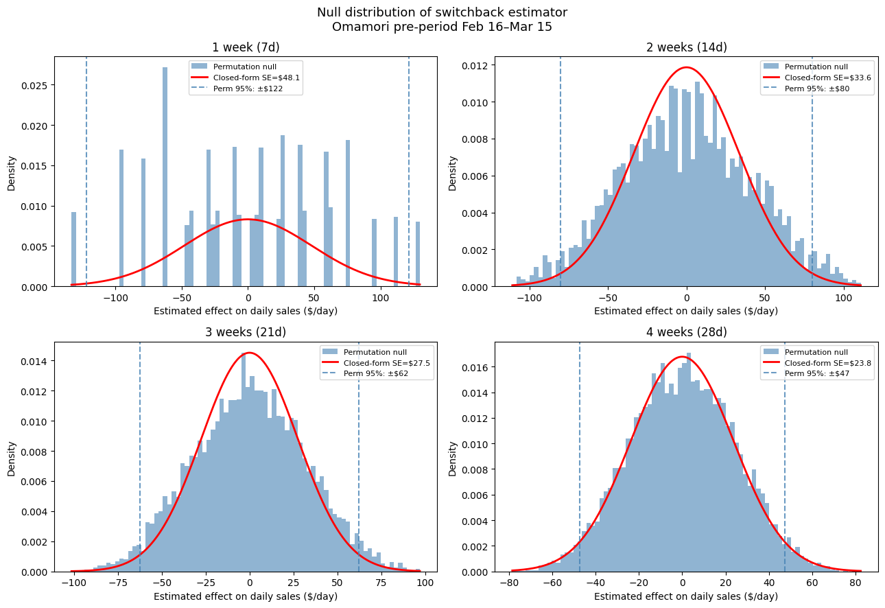
I then ran block-randomized permutation tests, simulating blocked assignment using 14-day blocks, 10,000 simulations for each time horizon, to generate the empirical distribution of the effect size under the null. Then I plotted these against the normal distribution the closed-form solution predicts.

When the math fails

Look at the one-week panel. The empirical distribution is a highly discrete, jagged mess. This is a combinatorics constraint: choosing 3 treatment days out of a 7-day block yields only 35 possible schedules. The empirical permutation standard error of $62.00 is a massive 29% higher than the closed-form expectation of $48.06.

But the two-week panel is where the real lesson lies. At 14 days we have 3,432 combinations, plenty of room for a continuous approximation. Yet the empirical standard error of $40.95 is still massively inflated compared to the closed-form expectation of $33.63, a ratio of 1.22.

Why? Day-of-week seasonality. The closed-form formula assumes every day is identical. But when you randomly assign 7 days to treatment out of 14, you can easily load up on high-sales weekends in one arm and low-sales weekdays in the other. The i.i.d. assumption is severely violated, and the theoretical math drastically understates the true variance of your estimator.

Convergence

1 week:   Perm SE $62.00 | CF SE $48.06 | Ratio 1.29
2 weeks:  Perm SE $40.95 | CF SE $33.63 | Ratio 1.22
3 weeks:  Perm SE $31.80 | CF SE $27.49 | Ratio 1.16
4 weeks:  Perm SE $24.18 | CF SE $23.78 | Ratio 1.02

By four weeks the empirical distribution has smoothed out to match the theoretical expectation. This happens because 28 days represents two full 14-day blocks, so the blocking design effectively balances the day-of-week effects and the autocorrelation is largely neutralized.

To translate that variance into business dollars: cutting bids by 50% gives expected daily ad cost savings of $13.51, and at a 50% gross margin my break-even threshold is a $27.03 drop in daily sales. At one week, the 95% confidence interval is incredibly wide at [−$53.01, $78.38], and 36.4% of simulations produce an estimate implying negative net profit. At four weeks it tightens to [−$9.62, $37.15], and misleading negative estimates drop to 13.3%.

The takeaway

If you rely on standard closed-form power calculators to size a time-series experiment, you may severely underestimate your variance and overestimate your statistical power. Permutation testing on pre-experiment data is an important diagnostic step. It quantifies exactly how much temporal autocorrelation inflates your variance, and it validates empirically when your blocking design has corrected for it.